If you've ever built an autonomous AI agent, you know the #1 production headache: how do you know your bot isn't tangled up in third-party API calls right now, feeding a customer polite nonsense? The textbook approach pushed by most trendy tutorials is blunt: grab the conversation logs (traces), ship them to a heavy flagship model like GPT-4o or Claude Opus with a prompt like "Rate whether there was an error from 1 to 5," and hope for the best.
Now let's do the math. When an agent runs thousands of sessions a day, calling a full-sized LLM-as-a-judge on every single turn turns into a massive money pit. On top of that, you eat 3–5 seconds of latency on every evaluation check.
Engineer and eval practitioner Hamel Husain, along with Antaripa Saha, published a detailed breakdown of a better alternative: specialized decision models. These are compact, non-generative classifiers that don't ramble about the meaning of life—they just return a concrete error probability. We touched earlier on the non-generative Typesafe Jev model, and now we have fresh benchmark numbers on real production logs.
98 Production Traces and a Classifier Showdown
The researchers took a real-world task: 98 valid traces from a complex lodging search-and-booking agent. The dataset contained 61 actual failures (wrong tool arguments, bad dates, logic breakdowns) and 37 successful task completions.
They fed those traces into five current decision models:
- Perplexity Decider 1.1 (27B): delivered record-low cost—just $0.0082 to check all 100 sessions, with an F1-score of 0.79. The trade-off was noticeable average latency at 7.85 seconds.
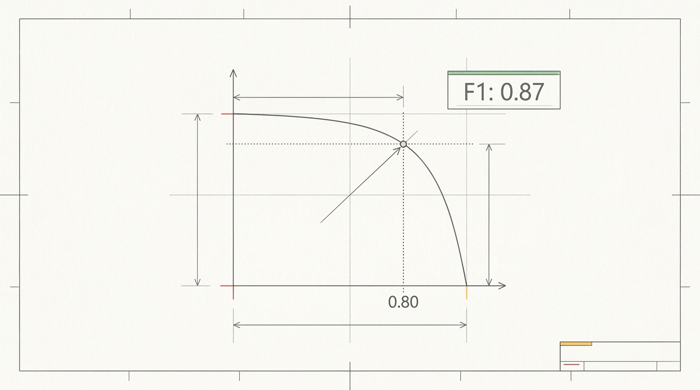
- OpenAI Decisions (powered by GPT-6 Luna): achieved the highest accuracy with an F1-score of 0.87, but cost $0.0372 per 100 runs—4.5x more expensive than Perplexity.
- Liquid d1 and d1-ultra: ultra-fast models with rock-bottom pricing ($0.02 and $0.042 per 1 million tokens) and response times of just 1.56 seconds.
- Cloudflare Clef Flash and TypeSafe Jev 1.13: solid lightweight classifiers with strict structured outputs.
The Default 0.50 Threshold Trap
The biggest takeaway from the study is that most teams throw money away because of a textbook habit. Once a classifier returns an error probability between 0.0 and 1.0, engineers slap on a default rule: "If the score is above 0.50, sound the alarm."
That's a fatal mistake. Raw model scores are biased: some architectures systematically underpredict, while others overpredict. At a 0.50 cutoff, Liquid d1 missed more than half of the real failures, whereas Perplexity Decider triggered a flood of false positives, forcing on-call engineers to mute Slack alerts.
In a real business, you're always balancing Precision (when an alert fires, is it actually a failure?) against Recall (what share of real failures did we catch?). To make the system predictable, you have to calibrate that cutoff mathematically.
Finding the Optimal Threshold in Python
Here is how you compute the best threshold from saved historical scores using scikit-learn. We enforce a strict business floor—both precision and recall must be at least 80%—and then maximize F1-score:
import numpy as np
from sklearn.metrics import precision_recall_curve

def find_optimal_threshold(y_true, y_scores, min_precision=0.80, min_recall=0.80):
    """
    Find a cutoff threshold that guarantees minimum precision and recall bounds.
    y_true: array of ground-truth labels (1 = error, 0 = success)
    y_scores: array of probabilities from the decision model
    """
    precisions, recalls, thresholds = precision_recall_curve(y_true, y_scores)
    best_threshold = 0.50
    best_f1 = 0.0

    for p, r, t in zip(precisions[:-1], recalls[:-1], thresholds):
        if p >= min_precision and r >= min_recall:
            # Compute harmonic mean of Precision and Recall
            f1 = 2 * (p * r) / (p + r) if (p + r) > 0 else 0.0
            if f1 > best_f1:
                best_f1 = f1
                best_threshold = float(t)

    return best_threshold, best_f1
Moving the cutoff from 0.50 to the calculated optimum (say, 0.38 for an under-confident model) immediately boosts F1-score by 10–15 points without fine-tuning weights or touching a single prompt.
Calibrating Probabilities with Platt Scaling
The second issue with raw models is distorted absolute values. If a model outputs 0.90, that doesn't mean 90 out of 100 cases are actually errors. To align those probabilities with reality, Platt scaling works great—fitting a logistic regression on top of the log-odds:
from sklearn.linear_model import LogisticRegression

def calibrate_platt_scaling(train_scores, train_labels, test_scores):
    """
    Calibrate classifier outputs using Platt scaling.
    Maps raw scores to honest statistical probabilities.
    """
    eps = 1e-6
    # Clip extreme values for log stability
    clipped_train = np.clip(train_scores, eps, 1.0 - eps)
    log_odds_train = np.log(clipped_train / (1.0 - clipped_train)).reshape(-1, 1)

    calibrator = LogisticRegression(C=1.0, solver='lbfgs')
    calibrator.fit(log_odds_train, train_labels)

    clipped_test = np.clip(test_scores, eps, 1.0 - eps)
    log_odds_test = np.log(clipped_test / (1.0 - clipped_test)).reshape(-1, 1)

    # Return calibrated probability for the positive class
    return calibrator.predict_proba(log_odds_test)[:, 1]
Platt scaling dramatically improves Brier score for systematically biased models (Perplexity, Liquid d1), but on tiny datasets (fewer than 50 examples) you risk overfitting. Always lock in a held-out test split before fitting the calibrator weights.
Bottom line: stop burning heavy LLMs on routine step-by-step agent checks. Pairing a fraction-of-a-cent decision model with a properly calibrated cutoff gives you the same reliability while saving both your budget and your support team's sanity.